Eric Bogatin's Signal Integrity Academy Blog

Figures of merit are single numbers that characterize important features in a large collection of data. They are incredibly powerful in taking a complex behavior and boiling it down to just a few special values. This makes understanding the behavior and comparing one system to another much easier.

Being aware of, and knowing how to use, figures of merit correctly are important elements in faster time to insight.

In this short column, we’ll look at a few figures of merit that characterize a time domain signal. As the example, we’ll use a sine wave signal I measured using my Teledyne LeCroy WavePro HD scope.

Figure . An example of the measured signal for this analysis on an expanded, zoomed scale.

The first step in looking at any measured results in a scope is “Situational Awareness.” This means knowing the details of the important limitations of your scope and the possible impact these limitations have on extracting accurate information from your signal. At the very least, this means being aware of the resolution of the scope in voltage and time.

The vertical resolution of the WavePro HD is 12-bits all the time. With 4 V full scale and 4096 levels in this span, the vertical resolution is about 1 mV per digitized level. This is a resolution of 1 mV out of about 2 V signal or 0.05% per bit level.

Since the period of this wave is 20 usec, and I want at least 1000 samples per cycle so I have adequate time resolution. This is a good criterion for general use. Unless I have a strong compelling reason otherwise, for example, if I want to see a very fast transient, or the rise time I want to measure is really short, 1000 samples per cycle is a good measurement goal. And, with deep memory in the WavePro HD, running out of memory for long acquisition sweeps is never a problem.

To measure this sine wave, I need at least 1000 Samples/20 usec = 50 MS/sec sampling rate in the digitizer. That was the minimum sample rate I used for this measurement. However, the WavePro HD scope is capable of so much more.

I took advantage of the large acquisition memory depth and actually used 5 msec per acquisition sweep. This is a total number of samples in the acquisition sweep of 50 MS/sec x 0.005 sec = 250k samples. This gives much better statistics when calculating figures of merit which get extracted per cycle. The more cycles we average, the better the statistics.

When we take a long acquisition sweep, we can’t see anything useful on the front screen, as shown here:

Figure . The measured data in on acquisition sweep with 250k samples.

To get the best of both worlds, I measured a deep memory acquisition sweep in which I did all the figure of merit calculations and then zoomed out on this window to see the individual cycles more clearly. The bright yellow region is the section that I zoomed.

Once we have data in an acquisition sweep, we can take advantage of a built-in parameter calculator to extract all the important figures of merit of the waveform automatically, at high resolution, in voltage and time, over many cycles.

You can watch me take this data and calculate the important figures of merit in this YouTube video.

As a source, I used a simple, low cost function generator I bought from eBay for $13.

Figure . Low cost function generator supplying the sine wave signal.

The seven most important figures of merit for a repetitive time domain signal are:

Frequency. This is how many times per second the signal repeats

Period: this is the time interval over which the pattern repeats. The period = 1/frequency

Amplitude: for an ideal sine wave, this is how much above the average and how much below the average the signal extends. However, this figure of merit is only of value for sine waves which are symmetric about their average. A more general figure of merit is the peak-to-peak value.

Peak-to-Peak: the (maximum value – the minimum value) over the entire period. For the case of a sine wave, it is 2 x amplitude. This term is more generic than an amplitude which is specific to a sine wave.

Average: is defined as

It is a measure of the offset or centered value of the waveform over some period of time. In our scope, this single figure of merit is calculated over the entire acquisition window of 5 msec. As long as we include many cycles, the effect of missing a fraction of a cycle is a tiny error.

At a minimum, as long as the average is calculated over a multiple of repeat periods, the average value is independent of the amount of time we average.

RMS (root mean square): is the square root of the average of the square of the waveform. Just as the average is the average of the voltage itself, the rms is the average of the square of the waveform, and then take the square root. It has units of voltage.

This is so important because the power generated by the signal, if it were to pass through a resistor, is related to the square of the rms voltage. The rms value is an important figure of merit about power dissipation. It is defined as

This is calculated over the entire acquisition sweep of the signal. At a minimum, as long as the rms is calculated over a multiple of repeat periods, the rms value is independent of the amount of time we calculate the rms.

In the special case of a sine wave, the rms value is calculated as

This means that if the average is 0, the rms value is just 0.707 x the amplitude. This is the well know relationship for the rms value of a sine wave.

However, if there is a DC offset to the sine wave, the rms value depends on the offset. In fact, it doesn’t matter if the offset is positive or negative, the rms value increases over just that due to the sine wave. This is important to keep in mind.

Often times, when we want to characterize a noise level using the rms value, especially if it is low level, the RMS value can be a misleading figure of merit. A DC component to the noise contributes to the rms value, in addition to the fluctuations we want to characterize. This means rms is not a good figure of merit for noise level. Just the fluctuations about the average could be measured if we were to first subtract off the average value then calculate the rms. That is exactly what the standard deviation term does.

Standard deviation: is defined as:

It is a measure of the distribution of the data about the mean or average. A large standard deviation, compared to the average, means the signal is varying all over the place. A small value of standard deviation, compared to the average, means the variation in the signal is very tightly distributed around the average.

In the entire acquisition window, we first calculate the average value. Then we go back through the data and calculate the square of the difference between the voltage and the average value. We add up all these squared deviations from the average and then find the average of them. To bring us back to voltage we take the square root.

The standard deviation is basically the rms value with the DC component subtracted off. The standard deviation has significance in a few special waveforms. When there is just noise, the standard deviation is a good figure of merit of the noise level. When I want to calculate a figure of merit for the noise level in an otherwise constant signal, the standard deviation is a much better figure of merit than the rms value.

In the special case of a Gaussian distribution of values, where the signal is centered about an average, the standard deviation calculated this way is exactly the standard deviation of the distribution. This term, along with the average, are the only terms needed to replicate the Gaussian distribution.

In the special case of a sine wave signal, the standard deviation is the rms of just the sine wave component:

Some of these figures of merit we can roughly read off the front screen of the scope. And, in fact, this is always an important first step. Adjusting the scales in which we display the data to convenient units makes this process so much easier.

However, the real power of a high-performance scope is unleashed when we can extract figures of merit of a signal using the 12-bit all the time vertical resolution, the fast sampling and the deep memory.

In our WavePro HD scope, we take advantage of these features by using a rich selection of built in parameter calculations. Watch this YouTube video to see how I calculate these important figures of merit for the sine wave example.

Once set up, we can display on the front screen the values of these important figures of merit, and their statistics: the average value, the min and max, and even their standard deviation. Here is an example of a snapshot of these automatic calculations extracted from each sweep of the acquisition window of 250k sample:

Example of the automatically measured figures of merit with the WavePro HD scope for this sine wave signal.

We should always look at the results and see if they are consistent with what we expect. The amplitude in this case is ½ the peak to peak value, or 1.01 V. We would expect a standard deviation value of 0.707 x 1.01 V = 0.714 V. We measure a standard deviation of 0.700 V. This is lower than 2% than we expected. How come?

We are assuming that the signal we measure is an ideal sine wave. In fact, it is close to an ideal sine wave, but is a little distorted. The lower standard deviation than expected is a small indication this signal is not an ideal sine wave.

Using these figures of merit are empirical. They are calculated based on the definitions above. It is up to us to interpret these values based on the type of signal we measure. They don’t tell us everything about this waveform, just a few terms that characterize it. We can gain even more insight into a signal by looking in the frequency domain. But that’s another story.

You’re an engineer if…

You see a problem and your fingers itch to fix it.

You see a finely working machine and you think about how you could make one even better.

You have ever used a paperclip, a coat hanger and duct tape for other than clipping paper, hanging things and taping ducts.

If the sales people at Best Buy can’t answer your questions about the computer you want to buy.

If you think the real heroes of Apollo 13 were the mission controllers who figured out a solution to the Co2 filter with duct tape and file folders.

If, when you were a kid, you were diagnosed with “the knack.”

Note sure what the knack is, watch this video:  https://youtu.be/g8vHhgh6oM0

I think a significant reason why some aspects of engineering are so confusing to many is because we get sloppy with the words we use. Changing our habits will make us all less confusing and increase the signal to noise ratio in the industry.

Here are six examples of terms we use all the time, yet they inspire confusion and shaking of heads when casually dropped. The same word means different things to different folks. Let’s take a look at some of the qualifiers we should get in the habit of using. When we hear or see these words, don’t hesitate to ask for clarification.

Let’s look at “bandwidth”, “impedance of an interconnect”, “inductance”, “ground”, “speed”, and “insertion and return loss”.

Bandwidth

Generally, bandwidth relates to the highest sine-wave frequency component that is significant. The confusion stems from what do we mean by “significant” and that bandwidth can refer to a signal, an interconnect, a measurement, and a model.

Bandwidth of a signal: The highest sine-wave frequency component in the signal, compared to an equivalent ideal square wave; usually the frequency at which the amplitude is below -3 dB of the square wave’s amplitude. Related to the rise time in the signal. To relate the bandwidth of a clock frequency, we are really making an assumption about the rise time of the clock signal.

Bandwidth of an interconnect: The highest sine-wave frequency that can be transmitted down the interconnect with acceptable attenuation. This is so dependent on the spec of what is acceptable. It is less ambiguous to refer to the -3 dB bandwidth of the interconnect, or the -10 dB bandwidth. This is unambiguous.

Bandwidth of a measurement: The highest sine-wave frequency component that is contained in the measurement. Easy to define for a frequency domain measurement, ambiguous for a time domain measurement. We usually define the -3 dB bandwidth of a measurement system as the frequency at which the measured frequency component is reduced to -3 dB of the input signal.

Bandwidth of a model: The highest sine wave frequency where the predictions of the model still match the actual measured response of the structure being modeled. How good the match is is very vague. Usually it is when the plotted simulation response is a few pen widths off from the measured response.

Impedance of an interconnect

Generally, impedance is always the ratio of a voltage to a current. But there are four different types of impedance relating to an interconnect.

Input impedance in the frequency domain: This is the impedance, at each frequency, looking between the signal and return connections at the front of the interconnect. At each frequency, the input impedance is about the total, complete, integrated effects from the entire interconnect including how it is terminated at the end. For an open transmission line, will look capacitive at low frequency and show the resonances of a typical transmission line.

Input impedance in the time domain: This is based on what a TDR might record. The initial input impedance will be the characteristic impedance, or a uniform transmission line, but only for a time less than the round trip time. After this time, there may be reflections which cause the input impedance to vary widely, ending up eventually at the impedance of the far end termination.

Instantaneous impedance of the transmission line: the impedance a signal will see each step along the way as it propagates down the transmission line. Will be constant if the cross section of the line is constant.

Characteristic impedance: Only applied to a uniform transmission line and is the one value of instantaneous impedance a signal will see on the transmission line. The one value of instantaneous impedance “characterizes” the transmission line.

Inductance

Generally, inductance is the number of magnetic field line rings surrounding a conductor per amp of current through the inductor. It is a property of the geometry of the conductors.

Loop-self-inductance: Refers to a conductor in a complete loop, as the total number of rings of magnetic field lines around the conductor per amp of current in that loop.

Loop-mutual-inductance: Refers to two conductors each as complete loops, as the total number of rings of magnetic field lines around one conductor produced by the current in the other conductor, per amp of current.

Partial-self inductance: The number of rings of magnetic field lines around a part of a loop, per amp of current in that loop. Cannot be directly measured, but can be calculated mathematically.

Partial-mutual inductance: The number of rings of magnetic field lines around a part of a loop, per amp of current through another part of the loop. Cannot be directly measured, but can be calculated mathematically.

Total inductance: the total number of rings of magnetic field lines around a part of a loop from all the currents contributing magnetic field lines, usually the partial self-inductance of the section, minus the partial mutual to all other parts of the loop. Can be measured from the voltage generated from a dI/dt through the section of conductor.

Ground

Generally a specific conductor identified in a system based on how it is used.

Circuit ground. Generally, the circuit nodes or terminals which are the lowest voltage point in a unipolar supplied circuit, or the mid voltage point in a bipolar power supplied circuit. It is from this conductor that the voltage on other nodes is measured relative to. Other than being the reference conductor, there is nothing special about the circuit ground.

Digital ground. Usually the circuit ground conductor which is the return path for the digital signals. The return path can also be a conductor with a DC voltage on it.

Analog ground. Usually the circuit ground conductor which is the return path for analog signals. Other than extreme cases where fractions of a mV DC drop are important, analog and digital ground can be the same conductor if a continuous plane is used. The return currents will remain separate in the plane, following the location of the signal line. The idea of separating analog and digital ground applies when the return path is not a plane, like leads in a connector or pins in a package. In these cases, ground bounce from digital signals can create huge cross talk on the analog signals.

Chassis ground. This is the metal housing associated with the product. It often provides shielding to reduce EMI. It also acts as a safety shield to product any user who might touch the chassis. Cable shields should be connected to the chassis ground in order to reduce common currents on the shield. In this case, the cable shield becomes an extenuation of the chassis. Usually the circuit ground of the board is connected to the chassis ground at one point. If multiple points are used, there may be some low frequency return currents flowing in the chassis. Of course, if the enclosure is plastic, there is no chassis ground.

Earth ground. This is the connection that ultimately leads to a copper rod driven into the ground (literally) to provide a reference voltage throughout a house or building. This is a safety issue required by some building codes. The round hole in an AC outlet is connected to this copper rod. UL requires that chassis ground be connected to earth ground as a safety feature. Ground fault interrupter (GFI) sockets are designed to disconnect power to a device if more than a few micro amps of current from the low side of the power mains flows through the earth ground connection. Of course, a car, satellite or other portable device has no connection to earth ground.

Speed

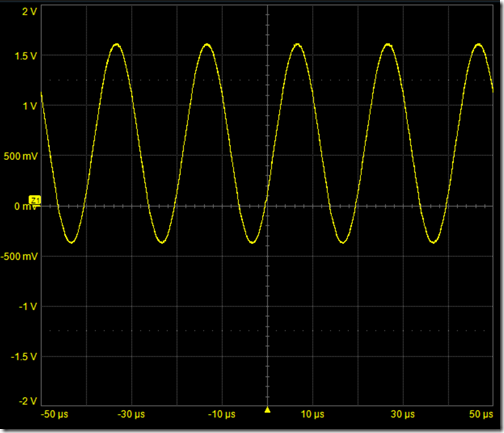
The speed of a signal is the most confusing term as it is used in two completely different contexts. Speed is generally related to the velocity of the signal. But it is also used to refer to the rate of data transfer.

Speed of light in air: about 1 foot per nsec, 12 inches/nsec, or 30 cm/nsec

Speed of light in most laminates. Since the Dk of most laminates is about 4, the speed of a signal in the laminate is about 6 inches/nsec or 15 cm/nsec

Speed of electrons in a conductor. Even in the extreme of cases, the speed of an electron in a copper wire is about 1 cm/sec, the speed of an ant. It has nothing to do with the speed at which an electric and magnetic field will propagate in a transmission line.

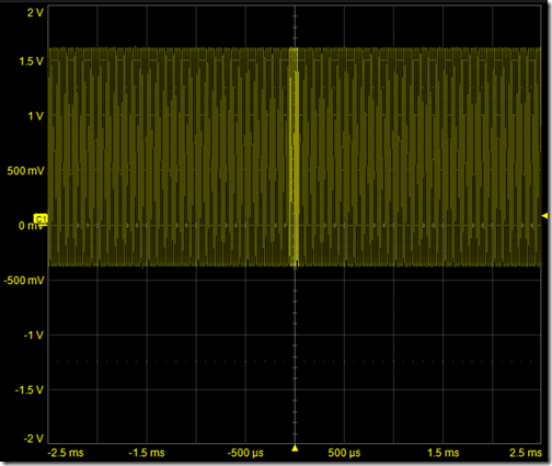
The clock frequency of a system: The frequency, usually in MHz, of the repetitive reference signal to synchronize system operations. The clock frequency of many high end microprocessors has increased over the last 30 years from 16 MHz. to 2.5 GHz.

The Nyquist frequency of a serial link signal: This is the frequency of the underlying clock of a serial link signal. It is the clock frequency when the data transition rate is the highest, 10101010101. This looks like a square wave and its frequency is the Nyquist. Since there are two bits per clock cycle, Double Data Rate (DDR), the Nyquist frequency is half the data rate. A 10 Gbps NRZ (non-return to zero) data pattern has a Nyquist of 5 GHz. The Nyquist and the encoding scheme, determine the maximum rate of data transmission in the channel, or the channel capacity.

The data rate of a serial link: The rate at which the data is transmitted as bits per second. In an NRZ pattern, with just two voltage levels for the signal, referred to as PAM2, each clock cycle has 2 bits of information encoded on it. The channel capacity for the data rate is twice the Nyquist frequency. If the Nyquist is 5 GHz, the data rate is 10 Gbps.

The baud rate. We often refer to the data content in a signal as the data payload. When an encoding scheme uses extra bits to carry routing information or synchronization information, not all the bits are payload data. We use the term baud rate to refer to the rate at which symbol transitions are transmitted. A symbol is the smallest unit of modulation. The data rate of Ethernet may be 10 Gbps but with a small percentage of the possible symbols being non-payload data, the actual transmission rate of symbols, the baud rate,  is 10.3125 Gbps.

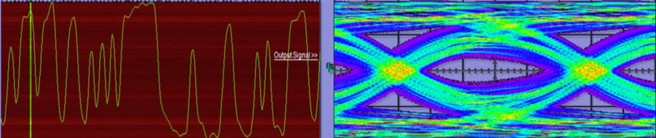
Insertion and return loss

These are throwback terms from the old days of how microwave measurements used to be performed. Two halves of a well matched fixture were measured separated and when connected together. When the device is inserted, the reflected signal and transmitted signal is measured.

The return loss is the loss in the returned signal of the open when the DUT is inserted. When open, all the signal returns. When the DUT is inserted, the better the match in the fixture, the less energy is returned; there is a large return loss, compared to an open. The larger the loss in the returned signal, compared to when the fixtures were open, the better the match.

The insertion loss is the ratio of the power received when the fixture is connected, compared with when the DUT is inserted. The less energy coming through the DUT, the more the insertion loss.

In both cases, the loss is defined as a positive dB value. The larger the value, the more loss. A large insertion loss means we lost a lot of signal when we inserted the DUT- not much gets through, not much is reflecting.

When we measure the S11 or S21 values of an interconnect, the magnitudes, in dB, are always negative for passive elements. Yet, we get in the habit of calling them return and insertion loss. To avoid the sign confusion, the industry is migrating to accepting return and insertion loss as either positive or negative.

The following terms apply to a uniform 2-port interconnect.

S11: the S-parameter = the reflection coefficient. The magnitude of S11, in dB, is the return loss, either as a positive or negative dB value. Referring to S11 as the reflection coefficient is unambiguous.

S21: the S-parameter = the transmission coefficient. The magnitude of S21, in dB, is the insertion loss, either as a positive or negative dB value. Referring to S21 as the transmission coefficient is unambiguous.

Attenuation = the attenuation in an interconnect, usually expressed in dB. It is usually a positive value. Larger values of attenuation in dB means more signal loss. Attenuation = -S21 in dB for a matched interconnect

Attenuation per length = dB/in or dB/m as a positive value.

These are just a few examples I encounter all the time. If we are not careful when we use these terms we leave confusion in our wake. Get in the habit of adding the qualifiers and it will help us communicate and think more clearly. Ultimately, we reduce the entropy in the universe and increase the signal to noise ratio in the industry.

I get this question all the time when we discuss dielectric loss in my classes. The common answer I get back is that this is the frequency for the resonance of a water molecule. It would make it the ideal frequency to run the oven so we get the most absorption.

But not always is the obvious answer the correct answer.

After all, is it a coincidence that 2.45 GHz is also the same frequency as 802.11ab wifi, the same as Bluetooth, and the Nyquist for PCIe gen 2, operating at 5 Gbps?

The use of 2.45 GHz is because this is in the center of the unlicensed ISM band of the FCC. One of the frequency bands of the Industrial, Scientific and Medical (ISM) bands is from 2.4 GHz to 2.5 GHz. This band is reserved for non telecommunications applications and does not require an FCC certification of compliance.

If you use this band for communications, buyer beware. Your protocol must be robust to interference and the FCC will not help patrol emissions in this frequency range.

If microwave ovens use this band so they don’t have to be certified by the FCC, how is it related to heating water?

The frequency of 2.45 GHz is a wavelength in air of 122 mm or 12.2 cm. When we look at the absorption spectrum of liquid water, the frequency is usually reported as the wavelength, instead.

This low frequency is well below the energy of vibration bands, and is more related to the loose, rather “fluid” lattice of the water molecules, smeared out due to fluctuating hydrogen bonding. Here is a typical absorption curve for liquid water, from 0 degC to 100 degC. There is a broad peak in the dissipation factor, around 3 cm which increases in frequency as temperature goes up.

Note that 12.2 cm, the wavelength of the microwave oven, is the black line. At 0 decC, the absorption of liquid water, the blue curve that is a measure of the dissipation factor, is actually sitting on the tail of the peak. It’s a very broad peak. As the water heats up, the absorption peak actually moves to higher frequency, shorter wavelength and the absorption for water actually gets worse.

The broad absorption by water, in the frequency range from 1 GHz to 100 GHz, is an important issue. This says that as an interconnect polymer absorbs water from the humidity in the air, we would expect the losses in the material to increase. This is why the humidity sensitivity to the dielectric loss of a laminate material is an important metric.

But why a microwave oven works at 2.45 GHz is more about the FCC than about the absorption resonance of water.

Every signal integrity engineer should be bilingual- able to speak in both the time domain and the frequency domain. This applies to signals and to the electrical properties of interconnects.

The basis of translating between the time domain and the frequency domain is the FFT and inverse FFT. If you have not done so, you should sit down and calculate the FFT of an ideal square wave in the time domain to see what its spectrum is in the frequency domain. After you do one by hand and see the underlying principles, its not important to do others by hand. Instead, you can use various simulation tools.

As a review, Teledyne LeCroy has put together a  handy little chart with a dozen time domain waveforms and what they look like in the frequency domain, as an amplitude histogram, and as an autocorrelation. You can download this simple chart here.